Briefly About TabNet
- TabNet is a deep learning architecture developed by Google in 2019 for analyzing tabular data.
- In many competitions, including Kaggle, tree-based ensemble models like XGBoost and LightGBM usually dominate the leaderboards when it comes to tabular data analysis.
- While deep learning leads in analyzing unstructured data like images, text, and audio, tree-based methods have been winning in structured data analysis.
- The TabNet creators noticed this trend and proposed "a novel high-performance and interpretable deep learning architecture" that incorporates the advantageous characteristics of both deep learning and decision tree methodologies, effectively emulating the learning patterns observed in tree-based apporaches.
Academic Paper:
https://arxiv.org/pdf/1908.07442
Abstract:
We propose a novel high-performance and interpretable canonical* deep tabular data learning architecture, TabNet. TabNet uses sequential attention to choose which features to reason from at each decision step, enabling interpretability and more efficient learning as the learning capacity is used for the most salient** features. We demonstrate that TabNet outperforms other variants on a wide range of non-performance-saturated*** tabular datasets and yields interpretable feature attributions plus insights into its global behavior. Finally, we demonstrate self-supervised learning for tabular data, significantly improving performance when unlabeled data is abundant.
*canonical: 기본형 **salient: 핵심적인 ***non-performance-saturated: 성능 개선의 여지가 많이 남아있는 상태
Details:
The paper talks about 4 main contributions to the new canonical DNN architecture for tabular data:
1.
"TabNet inputs raw tabular data without any preprocessing and is trained using gradient descent-based optimization, enabling flexible integration into end-to-end learning."

- End-to-end learning?
- Refers to a deep learning approach where a single network learns all steps from input to output without manual feature extraction or intermediate processing stages.
- Minimizes human intervention and manual feature engineering.
- Model learns necessary features and representations by itself.
2.
"TabNet uses sequential attention to choose which features to reason from at each decision step, enabling interpretability and better learning as the learning capacity is used for the most salient features (see Fig. 1). This feature selection is instance-wise, e.g. it can be different for each input, and unlike other instance-wise feature selection methods like (Chen et al. 2018) or (Yoon, Jordon, and van der Schaar 2019), TabNet employs a single deep learning architecture for feature selection and reasoning.

- Above figure is TabNet's sparse feature selection exemplified for Adult Census Income prediction.
- We can see how TabNet uses sequential attention to predict the income: first learns from professional occupation related features in the first decision step, then moves on to investment-related features in the next step.
- "Sparse feature selection enables interpretability and better learning as the capacity is used for the most salient features."
3.
"Above design choices lead to two valuable properties: (i) TabNet outperforms or is on par with other tabular learning models on various datasets for classficiation and regression problems from different domains; and (ii) TabNet enables two kinds of interpretability: local interpretability that visualizes the importance of features and how they are combined, and global interpretability which quanitifies the contribution of each feature to the trained model."
4.
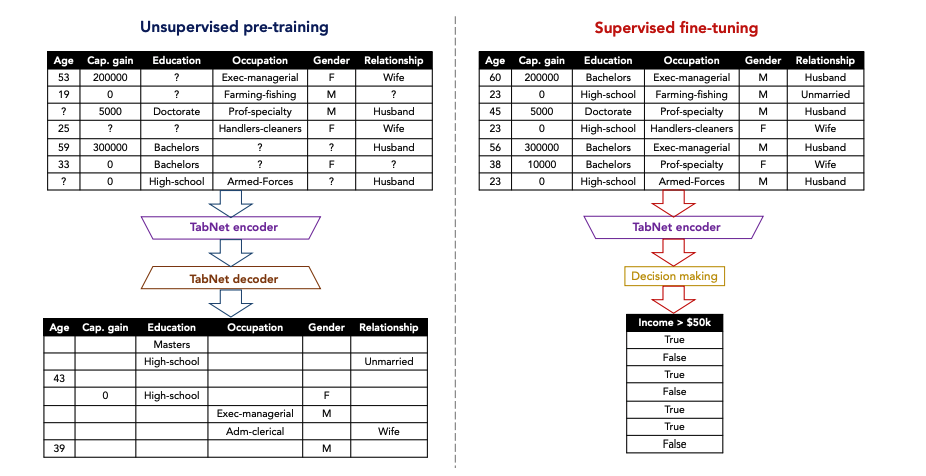
"Finally, for the first time for tabular data, we show significant performance improvements by using unsupervised pre-training to predict masked features (see Fig. 2)."

- Above figure identifies self-supervised tabular learning(자기 지도 학습).
- Self-supervised learning includes unsupervised pre-training and supervised fine-tuning in the figure.
- "Real-world tabular datasets have interdependent feature columns."
- The education level can be guessed from the occupation, or the gender can be guessed from the relationship."
- "Unsupervised representation learning by masked self-supervised learning results in an improved encoder model for the supervised learning task."
- Masking:
- technique of intentionally hiding parts of the data
- randomly hide parts of the original data; then train the model to predict the masked portions
- popularized by models like BERT
- Masking:
Architecture:

- Above figure is the illustration DT-like classification using conventional DNN blocks(left) and the corresponding decision manifold(right).
- If you check out the red mask boxes in the left image, you can see that in the first mask, only the first coefficient is set to 1 while everything else is 0. Then in the second mask, they set the second coefficient to 1.
- In other words, "relevant features are selected by using multiplicative sparse masks on inputs."
- This way, by zeroing out the weights of other feature, they are basically copying how decision trees work - making decision boundaries based on just the chosen features.
- "The selected features are linearly transformed, and after a bias addition (to represent boundaries) ReLU performs region selection by zeroing the regions".
- ReLu = max(0, x)
- selected features: x1, x2
- bias: b: [-aC1, aC1, -1, -1] & b: [-1, -1, -dC2, dC2]
- selected features are linearly transformed in the fully connected layer
- In other words, regions that don't meet certain conditions become zero and are excluded through ReLU(max(0,x))
- "Aggregation of multiple regions is based on addition."
- Final decision is made by summing the results from multiple regions
- Results from each branch(left and right) are added to create the final output
- Converted to final probability values through Softmax
- As C1 and C2 gets larger, the decision boundary gets sharper."
- C1 and C2 represent weight values
- the decision boundary gets sharper = the distinction between regions becomes more clear

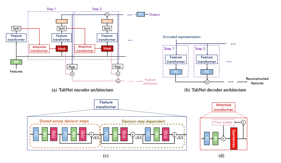
(a) TabNet encoder architecture
- TabNet encoder is composed of 1. feature transformer 2. attentive transformer and 3. feature masking.
- "A split block divides the processed representation to be used by the attentive transformer of the subsequent step as well as for the overall output. For each step, the feature selection mask provides interpretable information about the model's functionality, and the masks can be aggregated to obtain global feature important attribution."
- Basically means:
- In each step's Split block, the representation from the previous feature transformer gets sent in two directions: one to the output and another to the next attentive transformer.
- This helps sequentially learn the masks.
- By collecting all these learned masks together, you can figure out which features are important overall (global feature importance).
(b) TabNet decoder architecture
- TabNet decoder is composed of a feature transformer block at each step.
(c) Feature Transformer
- Above (c) figure is a feature transformer block example - "4 layer network is shown, where 2 are shared across all decision steps and 2 are decision step-dependent. Each layer is composed of a fully-connected (FC) layer, BN and GLU nonlinearity."
- BN:
- abbreviation of Batch Normalization, normalization technique engineered to stabilize and accelerate the training process of deep learning models
- TabNet uses Ghost Batch Normalization, a modification of conventional Batch Normalization technique, wherein the normalization process is executed by virtually partitioning larger batches into smaller constituent units, termed "ghost batches".
- GLU nonlinearity:
- abbreviation of Gated Linear Unit
- "nonlinearity" is added to emphasize that GLU functions is a nonlinear activation function rather than merely performing linear transformations
- The main purpose of this nonlinear activation function is to let the network decide how much information flows through a given path just as logical gate.
- IF we multiply 0, nothing passes.
- IF we multiply 0.3, 30% of the network flows.
- Multiplied value range between 0 and 1; therefore, we can use sigmoid function.
- The formula from the paper that introduces this idea is as below.
- First formula shows the details of the formula: we have two sets of weights (W and V), and two biases (b and c).
- Second formula indicates that the output of the linear mapping from the FC layer splits in two and fed into two parts: A into residual connection(direct linear transformation), B into sigmoid function. And then, multiply A and σ(B) element by element (⊗).
- paper reference: https://arxiv.org/pdf/1612.08083
- BN:


(d) Attentive Transformer
- Above (d) figure is an attentive transformer block example - "a single layer mapping is modulated with a prior scale information which aggregates how much each feature has been used before the current decision step. sparsemax is used for normalization of the coefficients, resulting in sparse selection of the salient features."
- "single layer mapping" includes Fully-connected layer(FC) and BN.
- Basically means:
- Attentive transformer makes masks using two things: 1. Prior scales and 2. Sparsemax.
- Prior sales keeps track of how much each feature has been used in previous steps.
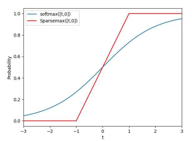
- Unlike softmax that distributes values across the entire domain, Sparsemax works more like Lasso or elasticnet in regression problems because it is more decisive, meaning that it marks important features as 1 and unimportant ones as 0 when creating masks.
- Softmax
- Turns all values into numbers between 0 and 1
- Every feature always gets some value(nothing gets totally ignored)
- Al values add up to 1
- Sparsemax
- splits feature values into 3 zones:
- 0: for features that don't matter much
- 1: for super important features
- Between 0 and 1: for somewhat important features(this is the sliding scale zone)
- Sparsemax has demonstrated superior performance when applied to sparse datasets, meaning that the data is scattered around with lots of gaps(0 value).
- Therefore, makes stronger choices about which features to use.
- Only picks features that are definitely important.
- Completely kicks out unnecessary features(sets them to 0).
- When we have more features, we get less 0~1 values(sliding scale zone) and fewer features end up getting the full 1 value.
- In other words, gets more picky (sparse) when there are more features to choose from.
- splits feature values into 3 zones:
- Softmax

- We need to train the sparse mask to pick out the important features from previous steps.
- Also, during the decision step process, we need to turn down the influence of variables that aren't really helpful for learning - we do this through masking technique.
- We use attentive transformer to make those masks: below formula shows how we get those masks.

- P[i] is calculated by multiplying (gamma - previous masks).
- This means that we're creating new masks by looking at both the features we've already processed in earlier decision steps, represented by a[i - 1], and the influence of previous masks, represented by P[i - 1].
- Gamma works like a flexibility control knob: when it is set to 1, it forces each feature to be used in just one decision step and as gamma gets bigger, it allows features to be used across multiple decision steps.
Conclusion:
- We should check DNN methods just as TabNet as well as conventional tree-based ensemble models to make better models.
- Even though TabNet is devised to get rid of preprocessing processes, it might still be better to manipulate dataset for better results.
- The paper was actually rejected by ICLR 2020 due to lack of experiments.
- However, there are Kaggle competitions that most of the baseline model of the top rankers was based on TabNet, which makes it evident that it is sufficiently powerful model.
Reference:
GLU: Gated Linear Unit
From paper to code
medium.com
Doubt is only removed by action. If you're not working, that's doubt being manifested.
- Conor Mcgregor -
'캐글' 카테고리의 다른 글
| [Kaggle Extra Study] 11. Polars (5) | 2024.11.06 |
|---|---|
| [Kaggle Study] 5. Regularization 가중치 규제 (3) | 2024.10.30 |
| [Kaggle Study] 4. Overfitting, Underfitting, Variance and Bias (4) | 2024.10.29 |
| [Kaggle Study] 3. Learning Rate (2) | 2024.10.29 |
| [Kaggle Study] 2. Scale of Features (1) | 2024.10.29 |