Loss Function
Machine learning algorithms find the patterns of the given dataset by themselves. For example, let's think about a situation that we should predict whether it will rain tomorrow or not from humidity data.
1.5 * x + 0.1 = y (raining if y > 1)
If we can simply express the relationship between the probability of rain and the humidity like this, "pattern" of this data is 1.5(weight) and 0.1(y intercept). We can call that equation "model" and the weight and the intercept is called the "model parameter".
Using the training dataset, model like above will be updated for better prediction performance. In the process of updating the model, we use "loss function" which is a standard of revising the "patterns" of the model.
Loss function simply defines the difference between prediction results and target value. Thus, we should think about how to minimize the difference(finding the minimum of loss function).
Linear Regression 선형 회귀
Linear regression is one of the most basic machine learning algorithms that models the linear relationship between train data(x) and target data(y).
Obviously, it aims to find a linear equation in the form of y = ax + b where a is the weight(slope) and b is the bias(intercept) of the model.
The purpose of linear regression is to use train data(x) and target data(y) to find weight(a) and intercept(b). In other words, the goal is to find an equation of line(직선의 방정식) which expresses the data best.
Gradient Descent is one of the methods to find that equation of line.
Gradient Descent 경사 하강법
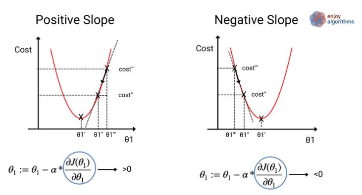
Gradient Descent is an optimization algorithm that uses the slope(rate of change) to upate the model so that it expresses the model better.
Gradient descent works well when the size of the data is large. However, gradient descent isn't the only way to solve regression problems: there are other methods such as normal equation(정규 방정식), decision tree(결정 트리), support vector machine, etc.

Brief process of gradient descent:
- Begin at some intial point on the linear equation(starting at a random point)
- Find the gradient(derivative) at the current position(tells us the direction of steepest increase)
- Move in the direction of the negative gradient
- Repeat: keep calculating gradients and continue until you reach a minimum where gradient gets close to 0
There are 3 main variants of gradient descent method:
- Stochastic Gradient Descent
- Uses only one data point per iteration to calculate the gradient.
- Pro:
- Fast learning speed
- Memory efficient
- Noise can help escape local minima and find better solutions
- Con:
- High variance in updates can make convergence unstable
- May not reflect characteristics of the entire dataset
- Batch Gradient Descent
- Uses the entire dataset to calculate the gradient
- Pro:
- Stable convergence
- Accurately reflects characteristics of entire dataset
- Suitable for parallel processing
- Con:
- Requires large memory
- Takes long time per update
- Can get stuck in local minima
- Mini-batch Gradient Descent
- Uses medium-sized batches(typically 32 ~ 256 samples)
- Pro:
- Balances benefits of both SGD and Batch GD
- Reasonable memory usage
- Stable yet fast learning
- Optimized for GPU utilization
- Con:
- Batch size becomes an additional hyperparameter
- Harder to escape local minima compared to SGD
Why we should shuffle order of samples in the training set for each epoch
- Shuffling the order of samples in the training dataset allows for diverse paths in the weight optimization process, making it more likely to find the optimal weights.
- One of the easiest ways to implement this is to shuffle the indices of numpy array and use those shuffled indices to call samples: np.random.permutation() method.
- It is far more efficient and fast this way.
indices = np.random.permutation(np.arrange(len(x)))
You can find more details about gradient descent from my previous posts:
ML/DL(2) - 오차 역전파(backpropagation)
'오차 역전파'라는 단어를 이해하는 것은 이 분야를 공부하면서 본인을 처음 흠칫하게 한 부분이었다. 나 같은 입문자가 이해하기 위해서는 부가적인 설명이 필요하다고 생각되는 부분이므로
dongsunseng.com
ML/DL(3) - 손실 함수와 경사 하강법의 관계
손실함수와 경사 하강법의 관계를 공부하며 헷갈리고 정확히 무슨말인지 이해가 안 가는 부분들이 있었는데 이들을 짚고 넘어가려 한다. 1. 왜 가중치와 절편을 업데이트하는데에 손실함수를
dongsunseng.com
Reference
Do it! 딥러닝 입문
★★★★★ 딥러닝을 배우고자 하는분께 강추합니다!(wtiger85 님) ★★★★★ 강추. 박해선님의 책은 일단 지른 다음에 생각합니다.(heistheguy 님) ♥♥♥♥ 코랩을 사용한 딥러닝을 알려주는 책 매
tensorflow.blog
Success is not determined by how many times you fall, but by how many times you get back up.
- Max Holloway -
'캐글' 카테고리의 다른 글
| [Kaggle Study] 2. Scale of Features (1) | 2024.10.29 |
|---|---|
| [Kaggle Study] #1 Titanic - Machine Learning from Disaster (2) | 2024.10.26 |
| ML/DL(3) - 손실 함수와 경사 하강법의 관계 (0) | 2023.07.08 |
| ML/DL(2) - 오차 역전파(backpropagation) (0) | 2023.07.08 |
| ML/DL(1) - 로지스틱 회귀의 활성화 함수로 비선형 함수를 사용하는 이유 (0) | 2023.07.08 |