CIBMTR - Equity in post-HCT Survival Predictions #4 GPU LightGBM Baseline [CV 681 LB 685)

This is an annotation of this kernel:

https://www.kaggle.com/code/cdeotte/gpu-lightgbm-baseline-cv-681-lb-685

GPU LightGBM Baseline - [CV 681 LB 685]

GPU LightGBM Baseline

In this notebook, we present a GPU LightGBM baseline. In this notebook, compared to my previous starter notebooks we teach 5 new things:

• How to tranform efs and efs_time into single target with KaplanMeierFitter.
• How to train GPU LightGBM model with KaplanMeierFitter target
• How to train XGBoost with Survivial:Cox loss
• How to train CatBoost with Survival:Cox loss
• How to ensemble 5 models using scipy.stats.rankdata().

Two Competition Approaches

In this competition, there are two ways to train a Survival Model:

• We can input both efs and efs_time and train a model that supports survival loss like Cox.
• Transform efs and efs_time into a single target proxy for risk score and train any model with regression loss like MSE.

• In this notebook, we train 5 models.
• The first 3 models (XGBoost, CatBoost, LightGBM) use bullet point two.
• And the next 2 models (XGBoost Cox, CatBoost Cox) use bullet point one. Discussion about this notebook is here and here.
• Since this competition's metric is a ranking metric, we ensemble the 5 predictions by first converting each into ranks using scipy.stats.rankdata().
• Afterward we created a weighted average from the ranks.

Previous Notebooks

My previous starter notebooks are:

• XGBoost and CatBoost starter here
• NN (MLP) starter here

Associated discussions are here, here, here

---

Pip Install Libraries for Metric

Since internet must be turned off for submission, we pip install from my other notebook here where I downloaded the WHL files.

!pip install /kaggle/input/pip-install-lifelines/autograd-1.7.0-py3-none-any.whl
!pip install /kaggle/input/pip-install-lifelines/autograd-gamma-0.5.0.tar.gz
!pip install /kaggle/input/pip-install-lifelines/interface_meta-1.3.0-py3-none-any.whl
!pip install /kaggle/input/pip-install-lifelines/formulaic-1.0.2-py3-none-any.whl
!pip install /kaggle/input/pip-install-lifelines/lifelines-0.30.0-py3-none-any.whl

• https://www.kaggle.com/code/cdeotte/pip-install-lifelines
• There is a discussion explaining how to use these WHL files here.
  • Annotation on the details posted on another blog of mine
• Below is a quick summary:
  • To compute the competition metric in your notebook, attached this notebook (which you are reading) which contains WHL files (because we need to pip install with internet off to be able to submit to comp).
•  Also attached Kaggle's metic notebook here.

Afterward to compute the competition metric, run this code where preds are your oof predictions:

from metric import score
y_true = train[["ID","efs","efs_time","race_group"]].copy()
y_pred = train[["ID"]].copy()
y_pred["prediction"] = preds
m = score(y_true.copy(), y_pred.copy(), "ID")
print(f"CV Score = {m}")

 

Load Train and Test

import numpy as np, pandas as pd
import matplotlib.pyplot as plt
pd.set_option('display.max_columns', 500)
pd.set_option('display.max_rows', 500)

test = pd.read_csv("/kaggle/input/equity-post-HCT-survival-predictions/test.csv")
print("Test shape:", test.shape )

train = pd.read_csv("/kaggle/input/equity-post-HCT-survival-predictions/train.csv")
print("Train shape:",train.shape)
train.head()

EDA on Train Targets

• There are two train targets efs and efs_time.
• When efs==1 we know patient had an event and we know time of event is efs_time.
• When efs==0 we do not know if patient had an event or not, but we do know that patient was without event for at least efs_time.

plt.hist(train.loc[train.efs==1,"efs_time"],bins=100,label="efs=1, Yes Event")
plt.hist(train.loc[train.efs==0,"efs_time"],bins=100,label="efs=0, Maybe Event")
plt.xlabel("Time of Observation, efs_time")
plt.ylabel("Density")
plt.title("Times of Observation. Either time to event, or time observed without event.")
plt.legend()
plt.show()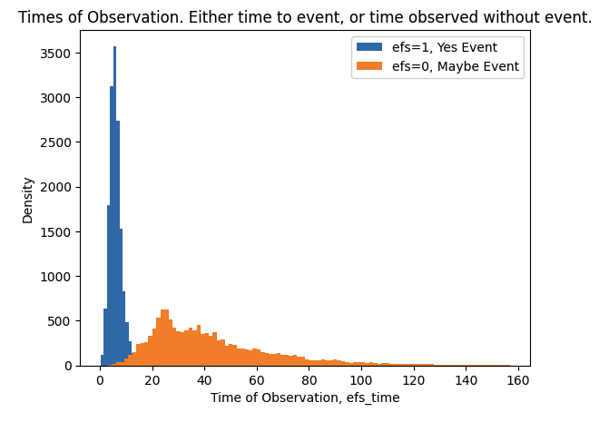

Transform Two Targets into One Target with KaplanMeier

• Both targets efs and efs_time provide useful information.
• We will tranform these two targets into a single target to train our model with.
• In this competition we need to predict risk score.
• So we will create a target that mimics risk score to train our model.
• (Note this is only one out of many ways to transform two targets into one target.
• Considering experimenting on your own).

from lifelines import KaplanMeierFitter
def transform_survival_probability(df, time_col='efs_time', event_col='efs'):
    kmf = KaplanMeierFitter()
    kmf.fit(df[time_col], df[event_col])
    y = kmf.survival_function_at_times(df[time_col]).values
    return y
train["y"] = transform_survival_probability(train, time_col='efs_time', event_col='efs')

plt.hist(train.loc[train.efs==1,"y"],bins=100,label="efs=1, Yes Event")
plt.hist(train.loc[train.efs==0,"y"],bins=100,label="efs=0, Maybe Event")
plt.xlabel("Transformed Target y")
plt.ylabel("Density")
plt.title("KaplanMeier Transformed Target y using both efs and efs_time.")
plt.legend()
plt.show()

Features

• There are a total of 57 features.
• From these 35 are categorical and 22 are numerical.
• We will label encode the categorical features.
• Then our XGB and CAT model will accept these as categorical features and process them special internally.
• We leave the numerical feature NANs as NANs because GBDT (like XGB and CAT) can handle NAN and will use this information.

RMV = ["ID","efs","efs_time","y"]
FEATURES = [c for c in train.columns if not c in RMV]
print(f"There are {len(FEATURES)} FEATURES: {FEATURES}")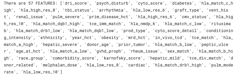

CATS = []
for c in FEATURES:
    if train[c].dtype=="object":
        CATS.append(c)
        train[c] = train[c].fillna("NAN")
        test[c] = test[c].fillna("NAN")
print(f"In these features, there are {len(CATS)} CATEGORICAL FEATURES: {CATS}")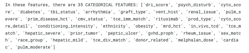

combined = pd.concat([train,test],axis=0,ignore_index=True)
#print("Combined data shape:", combined.shape )

# LABEL ENCODE CATEGORICAL FEATURES
print("We LABEL ENCODE the CATEGORICAL FEATURES: ",end="")
for c in FEATURES:

    # LABEL ENCODE CATEGORICAL AND CONVERT TO INT32 CATEGORY
    if c in CATS:
        print(f"{c}, ",end="")
        combined[c],_ = combined[c].factorize()
        combined[c] -= combined[c].min()
        combined[c] = combined[c].astype("int32")
        combined[c] = combined[c].astype("category")
        
    # REDUCE PRECISION OF NUMERICAL TO 32BIT TO SAVE MEMORY
    else:
        if combined[c].dtype=="float64":
            combined[c] = combined[c].astype("float32")
        if combined[c].dtype=="int64":
            combined[c] = combined[c].astype("int32")
    
train = combined.iloc[:len(train)].copy()
test = combined.iloc[len(train):].reset_index(drop=True).copy()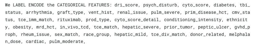

• Details about categorical feature label encoding part:
  • combined[c],_ = combined[c].factorize()
    
    • factorize() is a pandas function that converts categorical data like strings into numbers
    • Example: ['A', 'B', 'A', 'C'] → [0, 1, 0, 2]
    • '_' ignores the second return value (list of unique values)
  • combined[c] -= combined[c].min()
    
    • Subtracts the minimum value to make the sequence start from 0
    • Example: [1, 2, 1, 3] → [0, 1, 0, 2]
  • combined[c] = combined[c].astype("int32")
    
    • Converts data type to 32-bit integer
    • Used for memory efficiency
  • combined[c] = combined[c].astype("category")
    
    • Finally converts back to category type
    • For efficient handling of categorical data in pandas
      • Memory Efficiency
        • Category type internally stores repeating values as integers and maintains only a mapping table
        • Very efficient when strings like ['High', 'Low', 'High', 'Medium'] are repeated
      • Improved Operation Speed
        • Faster operations on categorical data
        • Optimized for tasks like grouping and sorting
      • Metadata Preservation
        • Explicitly expresses that this column is categorical
        • Better represents the meaning of the data
    • Result: Maintains information that this column is categorical, while saving memory
  • original = ['High', 'Low', 'High', 'Medium']
    ↓ factorize()
    [0, 1, 0, 2]
    ↓ No need to subtract min() (already starts from 0)
    [0, 1, 0, 2]
    ↓ Convert to int32
    [0, 1, 0, 2] (only data type changes)
    ↓ Convert to category
    [0, 1, 0, 2] (processed as categorical)

XGBoost with KaplanMeier

• Trained XGBoost model for 10 folds and achieved CV 0.674

from sklearn.model_selection import KFold
from xgboost import XGBRegressor, XGBClassifier
import xgboost as xgb
print("Using XGBoost version",xgb.__version__)

%%time
FOLDS = 10
kf = KFold(n_splits=FOLDS, shuffle=True, random_state=42) # shuffle=True for randomizing data
    
oof_xgb = np.zeros(len(train)) # out-of-fold predictions
pred_xgb = np.zeros(len(test)) # test data predictions

# k-fold cross validation loop -> Train on 90% and test(validation) on 10%
for i, (train_index, test_index) in enumerate(kf.split(train)):

    print("#"*25)
    print(f"### Fold {i+1}")
    print("#"*25)
    
    x_train = train.loc[train_index,FEATURES].copy()
    y_train = train.loc[train_index,"y"]
    x_valid = train.loc[test_index,FEATURES].copy()
    y_valid = train.loc[test_index,"y"]
    x_test = test[FEATURES].copy()

    model_xgb = XGBRegressor(
        device="cuda", # Use GPU
        max_depth=3,  # Tree depth
        colsample_bytree=0.5, # details below
        subsample=0.8,  # details below
        n_estimators=2000,  # Number of trees
        learning_rate=0.02,  
        enable_categorical=True, # Handle categorical variables
        min_child_weight=80, # details below
        #early_stopping_rounds=25,
    )
    
    model_xgb.fit(
        x_train, y_train,
        eval_set=[(x_valid, y_valid)],  
        verbose=500 
    )

    # INFER OOF: predictions for validation data
    oof_xgb[test_index] = model_xgb.predict(x_valid)
    
    # INFER TEST: predictions for test data
    pred_xgb += model_xgb.predict(x_test)

# COMPUTE AVERAGE TEST PREDS: Average predictions from 10 folds
pred_xgb /= FOLDS

1. colsample_bytree=0.5
   • Meaning: Proportion of features (columns) to use when creating each tree
   • Example:
     • If there are 100 features and colsample_bytree=0.5
     • Each tree uses only 50 randomly selected features
   • Effects:
     1. Prevents overfitting
     2. Tries various feature combinations
     3. Reduces over-dependence on specific features
   • Lower values: More conservative model, reduced overfitting risk
   • Higher values: Uses more features, can capture complex patterns
2. subsample=0.8
   • Meaning: Proportion of training data to use for each tree
   • Example:
     • If there are 1000 data points and subsample=0.8
     • Each tree learns from 800 randomly selected data points
   • Effects:
     1. Prevents overfitting
     2. Improves model generalization
     3. Ensures diversity as each tree learns from slightly different data
   • Lower values: More randomness, reduced overfitting risk
   • Higher values: Uses more data, stable learning
3. min_child_weight=80
   • Meaning: Minimum sum of weights required to create a leaf node
   • Example:
     • If min_child_weight=80
     • Won't split if the resulting node's weight sum would be less than 80
   • Effects:
     • Prevents splitting into too small groups
     • Controls overfitting
     • Improves model stability
   • Lower values: Allows finer splits, can learn complex patterns
   • Higher values: More conservative splits, reduced overfitting risk

Scoring the model:

from metric import score

y_true = train[["ID","efs","efs_time","race_group"]].copy()
y_pred = train[["ID"]].copy()
y_pred["prediction"] = oof_xgb
m = score(y_true.copy(), y_pred.copy(), "ID")
print(f"\nOverall CV for XGBoost KaplanMeier =",m)

feature_importance = model_xgb.feature_importances_
importance_df = pd.DataFrame({
    "Feature": FEATURES,  # Replace FEATURES with your list of feature names
    "Importance": feature_importance
}).sort_values(by="Importance", ascending=False)
plt.figure(figsize=(10, 15))
plt.barh(importance_df["Feature"], importance_df["Importance"])
plt.xlabel("Importance")
plt.ylabel("Feature")
plt.title("XGBoost KaplanMeier Feature Importance")
plt.gca().invert_yaxis()  # Flip features for better readability
plt.show()

CatBoost with KaplanMeier

• Trained CatBoost model for 10 folds and achieved CV 0.674

from catboost import CatBoostRegressor, CatBoostClassifier
import catboost as cb
print("Using CatBoost version",cb.__version__)

%%time
FOLDS = 10
kf = KFold(n_splits=FOLDS, shuffle=True, random_state=42)
    
oof_cat = np.zeros(len(train))
pred_cat = np.zeros(len(test))

for i, (train_index, test_index) in enumerate(kf.split(train)):

    print("#"*25)
    print(f"### Fold {i+1}")
    print("#"*25)
    
    x_train = train.loc[train_index,FEATURES].copy()
    y_train = train.loc[train_index,"y"]
    x_valid = train.loc[test_index,FEATURES].copy()
    y_valid = train.loc[test_index,"y"]
    x_test = test[FEATURES].copy()

    model_cat = CatBoostRegressor(
        task_type="GPU",  # Using GPU
        learning_rate=0.1,    
        grow_policy='Lossguide', # Details below
        #early_stopping_rounds=25,
    )
    model_cat.fit(x_train,y_train,
              eval_set=(x_valid, y_valid),
              cat_features=CATS,
              verbose=250)

    # INFER OOF
    oof_cat[test_index] = model_cat.predict(x_valid)
    # INFER TEST
    pred_cat += model_cat.predict(x_test)

# COMPUTE AVERAGE TEST PREDS
pred_cat /= FOLDS

• grow_policy='Lossguide'
  • Tree growth method: grow tree by selecting leaves that minimize loss

Scoring the model:

y_true = train[["ID","efs","efs_time","race_group"]].copy()
y_pred = train[["ID"]].copy()
y_pred["prediction"] = oof_cat
m = score(y_true.copy(), y_pred.copy(), "ID")
print(f"\nOverall CV for CatBoost KaplanMeier =",m)

feature_importance = model_cat.get_feature_importance()
importance_df = pd.DataFrame({
    "Feature": FEATURES, 
    "Importance": feature_importance
}).sort_values(by="Importance", ascending=False)
plt.figure(figsize=(10, 15))
plt.barh(importance_df["Feature"], importance_df["Importance"])
plt.xlabel("Importance")
plt.ylabel("Feature")
plt.title("CatBoost KaplanMeier Feature Importance")
plt.gca().invert_yaxis()  # Flip features for better readability
plt.show()

LightGBM with KaplanMeier

• Trained LightGBM model for 10 folds and achieved CV 0.6725

from lightgbm import LGBMRegressor
import lightgbm as lgb
print("Using LightGBM version",lgb.__version__)

FOLDS = 10
kf = KFold(n_splits=FOLDS, shuffle=True, random_state=42)
    
oof_lgb = np.zeros(len(train))
pred_lgb = np.zeros(len(test))

for i, (train_index, test_index) in enumerate(kf.split(train)):

    print("#"*25)
    print(f"### Fold {i+1}")
    print("#"*25)
    
    x_train = train.loc[train_index,FEATURES].copy()
    y_train = train.loc[train_index,"y"]    
    x_valid = train.loc[test_index,FEATURES].copy()
    y_valid = train.loc[test_index,"y"]
    x_test = test[FEATURES].copy()

    model_lgb = LGBMRegressor(
        device="gpu", 
        max_depth=3, 
        colsample_bytree=0.4,  
        #subsample=0.9, 
        n_estimators=2500, 
        learning_rate=0.02, 
        objective="regression", # detail below
        verbose=-1, # detail below
        #early_stopping_rounds=25,
    )
    model_lgb.fit(
        x_train, y_train,
        eval_set=[(x_valid, y_valid)],
    )
    
    # INFER OOF
    oof_lgb[test_index] = model_lgb.predict(x_valid)
    # INFER TEST
    pred_lgb += model_lgb.predict(x_test)

# COMPUTE AVERAGE TEST PREDS
pred_lgb /= FOLDS

• objective="regression"
  
  • Parameter that specifies the learning objective (loss function)
  • "regression" is the default setting for regression problems
  • Other options:
    • "binary": binary classification
    • "multiclass": multi-class classification
    • "ranking": ranking problems
    • "poisson": Poisson regression
    • "quantile": quantile regression
• verbose=-1
  
  • Specifies the level of detail for logs during training
  • Meaning of values:
    
    • -1: no output (completely silent)
    • 0: only warnings and errors
    • 1: basic information
    • 2: detailed information
  •  Currently set to -1, so no messages will be output during training

Scoring the model:

y_true = train[["ID","efs","efs_time","race_group"]].copy()
y_pred = train[["ID"]].copy()
y_pred["prediction"] = oof_lgb
m = score(y_true.copy(), y_pred.copy(), "ID")
print(f"\nOverall CV for LightGBM KaplanMeier =",m)

feature_importance = model_lgb.feature_importances_ 
importance_df = pd.DataFrame({
    "Feature": FEATURES,
    "Importance": feature_importance
}).sort_values(by="Importance", ascending=False)
plt.figure(figsize=(10, 15))
plt.barh(importance_df["Feature"], importance_df["Importance"], color='skyblue')
plt.xlabel("Importance (Gain)")
plt.ylabel("Feature")
plt.title("LightGBM KaplanMeier Feature Importance")
plt.gca().invert_yaxis()  # Flip features for better readability
plt.show()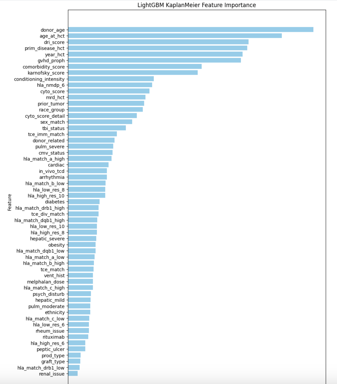

XGBoost with Survival:Cox

• Trained XGBoost using Survival:Cox loss for 10 folds and achieved CV=672!

# SURVIVAL COX NEEDS THIS TARGET (TO DIGEST EFS AND EFS_TIME)
train["efs_time2"] = train.efs_time.copy()
train.loc[train.efs==0,"efs_time2"] *= -1

• Above code prepares the target variable for Cox model
  • train["efs_time2"] = train.efs_time.copy()
    • Creates a new column by copying efs_time
  • train.loc[train.efs==0,"efs_time2"] *= -1
    • For cases where efs is 0 (no event occurred)
    • Converts the time value to negative
  • Reasons for doing this:
    
    • Cox models use this approach to represent censoring information
    • Negative time → censored case (no event occurred)
    • Positive time → event occurred case
  • Example:
    • Original Data:
      efs  | efs_time | efs_time2
      1    | 100      | 100      (death/relapse occurred)
      0    | 150      | -150     (censored)
      1    | 80       | 80       (death/relapse occurred)

FOLDS = 10
kf = KFold(n_splits=FOLDS, shuffle=True, random_state=42)
    
oof_xgb_cox = np.zeros(len(train))
pred_xgb_cox = np.zeros(len(test))

for i, (train_index, test_index) in enumerate(kf.split(train)):

    print("#"*25)
    print(f"### Fold {i+1}")
    print("#"*25)
    
    x_train = train.loc[train_index,FEATURES].copy()
    y_train = train.loc[train_index,"efs_time2"]    
    x_valid = train.loc[test_index,FEATURES].copy()
    y_valid = train.loc[test_index,"efs_time2"]
    x_test = test[FEATURES].copy()

    # same attributes with xgb above except objective and eval-metric
    model_xgb_cox = XGBRegressor(
        device="cuda",
        max_depth=3,  
        colsample_bytree=0.5,  
        subsample=0.8,  
        n_estimators=2000,  
        learning_rate=0.02,  
        enable_categorical=True,
        min_child_weight=80,
        objective='survival:cox',
        eval_metric='cox-nloglik',
    )
    model_xgb_cox.fit(
        x_train, y_train,
        eval_set=[(x_valid, y_valid)],  
        verbose=500  
    )
    
    # INFER OOF
    oof_xgb_cox[test_index] = model_xgb_cox.predict(x_valid)
    # INFER TEST
    pred_xgb_cox += model_xgb_cox.predict(x_test)

# COMPUTE AVERAGE TEST PREDS
pred_xgb_cox /= FOLDS

 

Scoring the model:

y_true = train[["ID","efs","efs_time","race_group"]].copy()
y_pred = train[["ID"]].copy()
y_pred["prediction"] = oof_xgb_cox
m = score(y_true.copy(), y_pred.copy(), "ID")
print(f"\nOverall CV for XGBoost Survival:Cox =",m)

feature_importance = model_xgb_cox.feature_importances_
importance_df = pd.DataFrame({
    "Feature": FEATURES,  # Replace FEATURES with your list of feature names
    "Importance": feature_importance
}).sort_values(by="Importance", ascending=False)
plt.figure(figsize=(10, 15))
plt.barh(importance_df["Feature"], importance_df["Importance"])
plt.xlabel("Importance")
plt.ylabel("Feature")
plt.title("XGBoost Survival:Cox Feature Importance")
plt.gca().invert_yaxis()  # Flip features for better readability
plt.show()

CatBoost with Survival:Cox

• Trained CatBoost using Survival:Cox loss for 10 folds and achieved CV=671!

FOLDS = 10
kf = KFold(n_splits=FOLDS, shuffle=True, random_state=42)
    
oof_cat_cox = np.zeros(len(train))
pred_cat_cox = np.zeros(len(test))

for i, (train_index, test_index) in enumerate(kf.split(train)):

    print("#"*25)
    print(f"### Fold {i+1}")
    print("#"*25)
    
    x_train = train.loc[train_index,FEATURES].copy()
    y_train = train.loc[train_index,"efs_time2"]    
    x_valid = train.loc[test_index,FEATURES].copy()
    y_valid = train.loc[test_index,"efs_time2"]
    x_test = test[FEATURES].copy()

    model_cat_cox = CatBoostRegressor(
        loss_function="Cox",
        #task_type="GPU",   
        iterations=400,   # Total number of trees to train  
        learning_rate=0.1,  
        grow_policy='Lossguide',
        use_best_model=False, # details below
    )
    model_cat_cox.fit(x_train,y_train,
              eval_set=(x_valid, y_valid),
              cat_features=CATS,
              verbose=100)
    
    # INFER OOF
    oof_cat_cox[test_index] = model_cat_cox.predict(x_valid)
    # INFER TEST
    pred_cat_cox += model_cat_cox.predict(x_test)

# COMPUTE AVERAGE TEST PREDS
pred_cat_cox /= FOLDS

• use_best_model=False
  
  • Uses all iterations (doesn't use early-stopped optimal model)
  • Conversely, when use_best_model=True:
    1. Selects the model from the point showing best performance on validation data
    2. Stops training if performance decreases in subsequent iterations
    3. Acts as a form of early stopping
  • Reasons for setting it to False:
    • Later iterations can sometimes be important in Cox models
    • Even if validation performance temporarily worsens, it might help overall survival prediction
    • Especially with lots of censored data, using all iterations might be more stable
  • Example:
    • # When True
      iter 100: performance 0.8
      iter 200: performance 0.85 (best)
      iter 300: performance 0.83
      → Uses model from iter 200
      
      # When False
      Uses combined results from all iterations (400)

Scoring the model:

y_true = train[["ID","efs","efs_time","race_group"]].copy()
y_pred = train[["ID"]].copy()
y_pred["prediction"] = oof_cat_cox
m = score(y_true.copy(), y_pred.copy(), "ID")
print(f"\nOverall CV for CatBoost Survival:Cox =",m)

feature_importance = model_cat_cox.get_feature_importance()
importance_df = pd.DataFrame({
    "Feature": FEATURES, 
    "Importance": feature_importance
}).sort_values(by="Importance", ascending=False)
plt.figure(figsize=(10, 15))
plt.barh(importance_df["Feature"], importance_df["Importance"])
plt.xlabel("Importance")
plt.ylabel("Feature")
plt.title("CatBoost Survival:Cox Feature Importance")
plt.gca().invert_yaxis()  # Flip features for better readability
plt.show()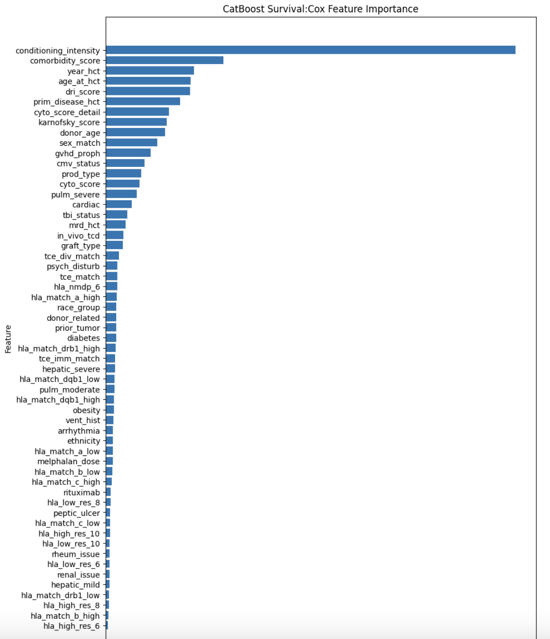

Ensemble CAT and XGB and LGB

• We ensemble our XGBoost, CatBoost, LightGBM, XGBoost Cox, and CatBoost Cox using scipy.stats.rankdata() and achieve an amazing CV=0.681 Wow!

from scipy.stats import rankdata 

y_true = train[["ID","efs","efs_time","race_group"]].copy()
y_pred = train[["ID"]].copy()
y_pred["prediction"] = rankdata(oof_xgb) + rankdata(oof_cat) + rankdata(oof_lgb)\
                     + rankdata(oof_xgb_cox) + rankdata(oof_cat_cox)
m = score(y_true.copy(), y_pred.copy(), "ID")
print(f"\nOverall CV for Ensemble =",m)

• rankdata: Function that returns the rank of each prediction -> Sums up ranks from five models
• How does the function work(Example):
• from scipy.stats import rankdata
  # Sample data
  predictions = [10.5, 5.2, 15.7, 5.2, 8.1]
  # Apply rankdata
  ranks = rankdata(predictions)
  
  1. First, sort the values in ascending order:
     • 5.2, 5.2, 8.1, 10.5, 15.7
       (1-2), (1-2), (3), (4), (5)
  2. Assign ranks to each value:
     • Original: [10.5,  5.2,  15.7,  5.2,   8.1]
       Ranks:    [4,     1.5,  5,     1.5,   3]
     • Since 5.2 appears twice, both receive 1.5 (average of 1st and 2nd place)
  3. Sum the rank value
     • model1_ranks = rankdata([0.1, 0.2, 0.3])  # [1, 2, 3]
       model2_ranks = rankdata([0.3, 0.1, 0.2])  # [3, 1, 2]
       ensemble = model1_ranks + model2_ranks     # [4, 3, 5]
• Why use rankdata? --> Suitable for Survival Analysis
  • Well-aligned with rank-based evaluation metrics such as the Concordance index
  • The relative risk ranking is often more important than the actual survival time

Create Submission CSV

sub = pd.read_csv("/kaggle/input/equity-post-HCT-survival-predictions/sample_submission.csv")
sub.prediction = rankdata(pred_xgb) + rankdata(pred_cat) + rankdata(pred_lgb)\
                     + rankdata(pred_xgb_cox) + rankdata(pred_cat_cox)
sub.to_csv("submission.csv",index=False)
print("Sub shape:",sub.shape)
sub.head()

---

Cast all your anxiety on him because he cares for you
<Peter 5:7>